Third-order Moment

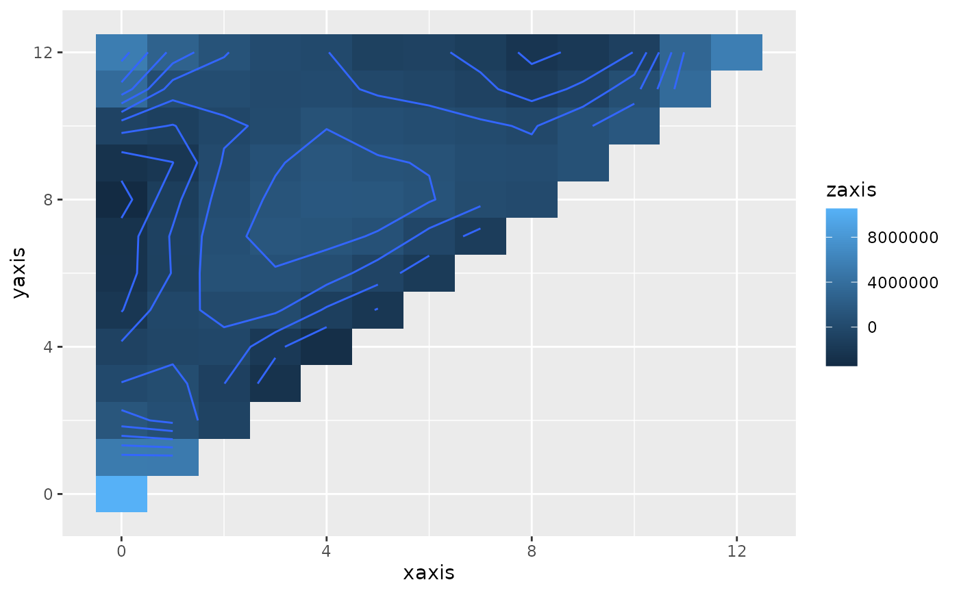
Estimated third order moment for a time series.

Usage

third(
  data,
  n.lag,
  centre = TRUE,
  outmax = TRUE,
  plot = lifecycle::deprecated()
)

Arguments

data: a vector of equally spaced numeric observations (time series).
n.lag: the number of lags, maximum = length of time series.
centre: centre series by subtracting mean (default=TRUE).
outmax: display the (x,y) lag co-ordinates for the maximum and minimum values (default=TRUE).
plot: Use autoplot.third() on the returned object instead. See examples.

Value

an object of class "third" (a list) with the following elements:

waxis: the axis from -n.lag to n.lag.
third: the estimated third order moment in the range -n.lag to n.lag, including the symmetries.
n.lag: the maximum lag.

Pass the result to autoplot() to draw the contour plot.

Details

The third-order moment is the extension of the second-order moment (essentially the autocovariance). The equation for the third order moment at lags (j,k) is: \(n^{-1}\sum X_t X_{t+j} X_{t+k}\). The third-order moment is useful for testing for non-linearity in a time series, and is used by nonlintest().

Author

Adrian Barnett a.barnett@qut.edu.au

Examples

# \donttest{
t <- third(CVD$cvd, n.lag = 12)
#> Maximum at (including symmetries):
#>   0 0
#> Minimum at (including symmetries):
#>   -8 8 0 -8 0 8
autoplot(t)

# }