Plot a Sinusoid — sinusoid • season

Plots a sinusoid over 0 to 2\(\pi\).

Usage

sinusoid(amplitude, frequency, phase)

Arguments

amplitude: the amplitude of the sinusoid (its maximum value).
frequency: the frequency of the sinusoid in 0 to 2\(\pi\) (number of cycles).
phase: the phase of the sinusoid (location of the peak).

Value

tibble of sinusoidal wave of given amplitude, frequency, and phase.

Details

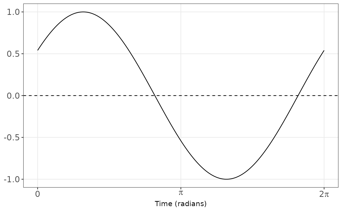
Sinusoidal curves are useful for modelling seasonal data. A sinusoid is plotted using the equation: \(A\cos(ft-P), t=0,\ldots,2 \pi\), where \(A\) is the amplitude, \(f\) is the frequency, \(t\) is time and \(P\) is the phase.

References

Barnett, A.G., Dobson, A.J. (2010) Analysing Seasonal Health Data. Springer. doi:10.1007/978-3-642-10748-1

Author

Adrian Barnett a.barnett@qut.edu.au

Examples

s_n <- sinusoid(
  amplitude = 1,
  frequency = 1,
  phase = 1
  )
s_n
#> # A tibble: 2,001 × 2
#>       time sinusoid
#>      <dbl>    <dbl>
#>  1 0          0.540
#>  2 0.00314    0.543
#>  3 0.00628    0.546
#>  4 0.00942    0.548
#>  5 0.0126     0.551
#>  6 0.0157     0.553
#>  7 0.0188     0.556
#>  8 0.0220     0.559
#>  9 0.0251     0.561
#> 10 0.0283     0.564
#> # ℹ 1,991 more rows
# plot it
autoplot(s_n)