Amplitude Adjusted Fourier Transform (AAFT)

Generates random linear surrogate data of a time series with the same second-order properties.

Usage

aaft(data, nsur)

Arguments

data

a vector of equally spaced numeric observations (time series).

nsur

the number of surrogates to generate (1 or more).

Value

a matrix of the nsur surrogates.

Details

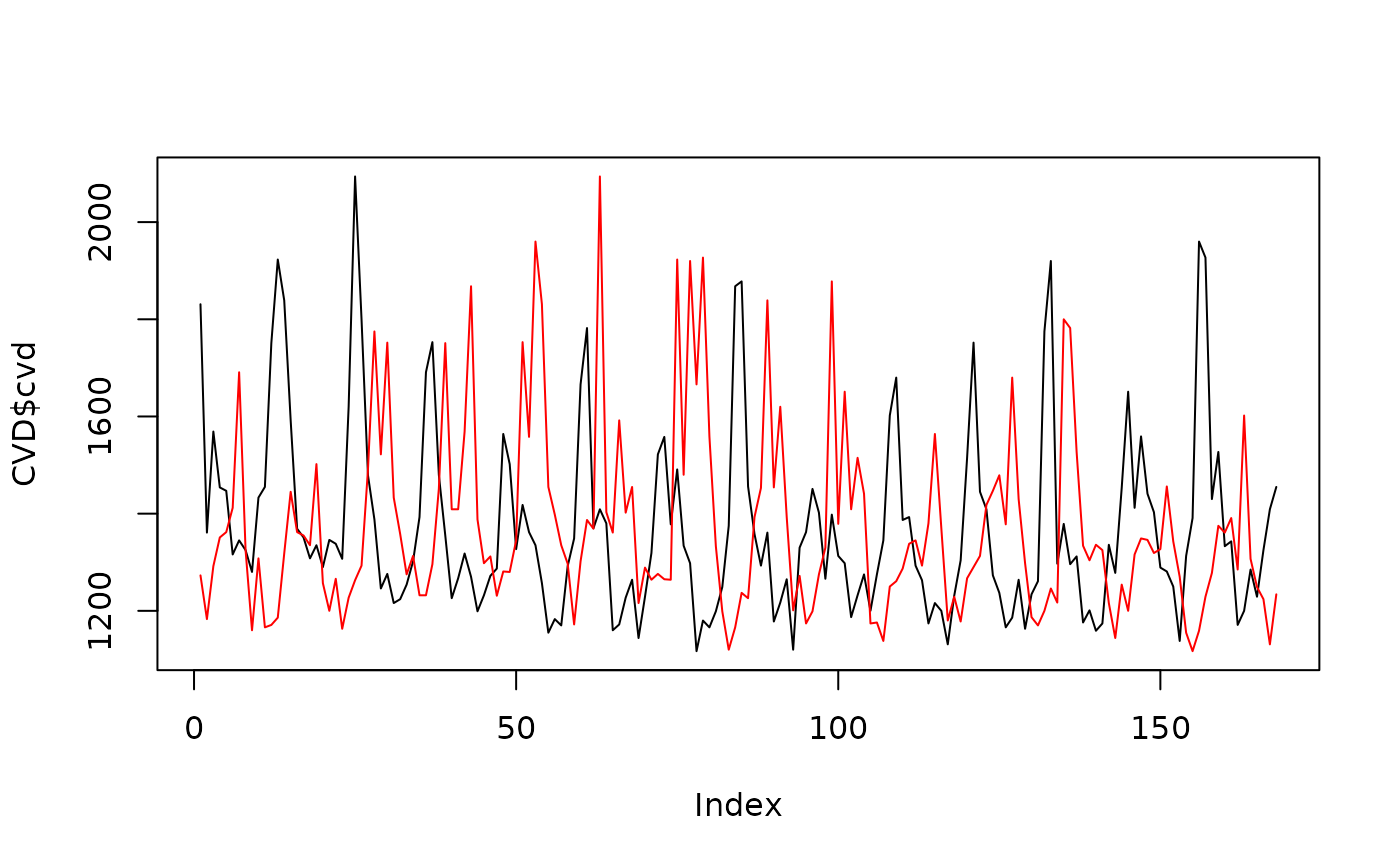
The AAFT uses phase-scrambling to create a surrogate of the time series that has a similar spectrum (and hence similar second-order statistics). The AAFT is useful for testing for non-linearity in a time series, and is used by nonlintest.

References

Kugiumtzis D (2000) Surrogate data test for nonlinearity including monotonic transformations, Phys. Rev. E, vol 62 no. 1, 2000. doi:10.1103/PhysRevE.62.R25

Author

Adrian Barnett a.barnett@qut.edu.au

Examples

# \donttest{
aaft(CVD$cvd, nsur = 1)
#>        [,1]
#>   [1,] 1263
#>   [2,] 1231
#>   [3,] 1138
#>   [4,] 1117
#>   [5,] 1325
#>   [6,] 1361
#>   [7,] 1960
#>   [8,] 1409
#>   [9,] 1375
#>  [10,] 1387
#>  [11,] 1333
#>  [12,] 1246
#>  [13,] 1160
#>  [14,] 1187
#>  [15,] 1232
#>  [16,] 1163
#>  [17,] 1409
#>  [18,] 1402
#>  [19,] 1782
#>  [20,] 1380
#>  [21,] 1451
#>  [22,] 1433
#>  [23,] 1261
#>  [24,] 1343
#>  [25,] 1176
#>  [26,] 1234
#>  [27,] 1159
#>  [28,] 1226
#>  [29,] 1346
#>  [30,] 1319
#>  [31,] 1455
#>  [32,] 1362
#>  [33,] 1388
#>  [34,] 1430
#>  [35,] 1249
#>  [36,] 1287
#>  [37,] 1200
#>  [38,] 1270
#>  [39,] 1297
#>  [40,] 1120
#>  [41,] 1172
#>  [42,] 1289
#>  [43,] 1592
#>  [44,] 1522
#>  [45,] 1775
#>  [46,] 1558
#>  [47,] 1355
#>  [48,] 1312
#>  [49,] 1171
#>  [50,] 1174
#>  [51,] 1174
#>  [52,] 1216
#>  [53,] 1264
#>  [54,] 1454
#>  [55,] 1752
#>  [56,] 1527
#>  [57,] 1393
#>  [58,] 1318
#>  [59,] 1201
#>  [60,] 1281
#>  [61,] 1250
#>  [62,] 1180
#>  [63,] 1216
#>  [64,] 1166
#>  [65,] 1200
#>  [66,] 1308
#>  [67,] 1923
#>  [68,] 1502
#>  [69,] 1412
#>  [70,] 1403
#>  [71,] 1296
#>  [72,] 1307
#>  [73,] 1183
#>  [74,] 1144
#>  [75,] 1345
#>  [76,] 1273
#>  [77,] 1200
#>  [78,] 1455
#>  [79,] 1927
#>  [80,] 1559
#>  [81,] 1393
#>  [82,] 1409
#>  [83,] 1275
#>  [84,] 1293
#>  [85,] 1232
#>  [86,] 1227
#>  [87,] 1292
#>  [88,] 1327
#>  [89,] 1298
#>  [90,] 1447
#>  [91,] 1839
#>  [92,] 1920
#>  [93,] 1751
#>  [94,] 1868
#>  [95,] 1753
#>  [96,] 1515
#>  [97,] 1224
#>  [98,] 1199
#>  [99,] 1335
#> [100,] 1265
#> [101,] 1325
#> [102,] 1302
#> [103,] 1878
#> [104,] 1569
#> [105,] 1445
#> [106,] 1456
#> [107,] 1361
#> [108,] 1351
#> [109,] 1358
#> [110,] 1229
#> [111,] 1275
#> [112,] 1290
#> [113,] 1334
#> [114,] 1620
#> [115,] 1680
#> [116,] 1831
#> [117,] 2094
#> [118,] 1666
#> [119,] 1378
#> [120,] 1313
#> [121,] 1369
#> [122,] 1336
#> [123,] 1266
#> [124,] 1229
#> [125,] 1330
#> [126,] 1564
#> [127,] 1800
#> [128,] 1418
#> [129,] 1491
#> [130,] 1441
#> [131,] 1338
#> [132,] 1480
#> [133,] 1155
#> [134,] 1278
#> [135,] 1237
#> [136,] 1217
#> [137,] 1267
#> [138,] 1362
#> [139,] 1691
#> [140,] 1651
#> [141,] 1602
#> [142,] 1398
#> [143,] 1272
#> [144,] 1285
#> [145,] 1178
#> [146,] 1166
#> [147,] 1257
#> [148,] 1131
#> [149,] 1293
#> [150,] 1349
#> [151,] 1479
#> [152,] 1370
#> [153,] 1379
#> [154,] 1345
#> [155,] 1254
#> [156,] 1276
#> [157,] 1170
#> [158,] 1264
#> [159,] 1298
#> [160,] 1199
#> [161,] 1280
#> [162,] 1316
#> [163,] 1453
#> [164,] 1391
#> [165,] 1313
#> [166,] 1335
#> [167,] 1186
#> [168,] 1304
surr <- aaft(CVD$cvd, nsur = 1)
plot(CVD$cvd, type = "l")
lines(surr[ ,1], col = "red")

# }